Introduction
What follows is an example I worked up when trying to figure out how to communicate potential outcomes in a regression framework to students graphically. This discussion is derived from Morgan and Winship’s 2015 book1, especially pages 122-123. The goal is to represent the potential outcomes framework using standard regression notation, and then to discuss endogenous selection bias using this framework.
Math
Define \(Y_i = \mu_0 + (\mu_1 - \mu_0)D_i + \{v^0_i + D_i(v^1_i-v^0_i)\}\) where \(D_i\) is binary assignment to treatment for individual \(i\), \(\mu_0\) is the expected outcome for control, \(\mu_1\) is the expected outcome for treated, \(\mu_1 - \mu_0\) is the Average Treatment Effect or \(\delta\). The \(v\) terms are subset by \(i\) denoting that they are individual heterogeneity. \(v^0_i\) is an individual’s deviation from \(\mu_0\) under control, or \(Y_i^0 = \mu_0 + v^0_i\). The same can be said for \(v^1_i\), it is an individuals deviation from \(\mu_1\) under treatment or \(Y_i^1 = \mu_1 + v^1_i\). Treatment minus control is equal to \((Y_i^1) - (Y_i^0) = (\mu_1 + v^1_i) - (\mu_0 + v^0_i)\) which is equal to the average treatment effect \(\mu_1 - \mu_0\) and the individual heterogeneity in the treatment effect \(v^1_i-v^0_i\).
For \(\mu_0\) to properly represent the mean of \(Y_i\) under control, the \(E[v^0_i]\) must be equal to zero, or \(\dfrac{\Sigma_i^N v^0_i}{N} = \Sigma_i^n v^0_i= 0\). You can get here from the linearity of expectation, such that if \(\mu_0 = E[Y_i]\) for control, we can substitute such that \(\mu_0 = E[\mu_0 + v^0_i] = E[\mu_0] + E[v^0_i] = \mu_0 + E[v^0_i]\), therefore \(E[v^0_i]=0\). The same is true for \(E[v^1_i]\), \(\mu_1 = E[\mu_1 + v^1_i] = E[\mu_1] + E[v^1_i] = \mu_1 + E[v^1_i]\). By the same token, then \(E[v^1_i - v^0_i]=E[v^1_i] - E[v^0_i]=0\).
Morgan and Winship argue that issues arise when “\(D_i\) is correlated with the population-level variant of the error term, \(\{v^0_i + D_i(v^1_i-v^0_i)\}\), as would be the case when the size of the individual-level treatment effect, in this case \((\mu_1 - \mu_0) + \{v^0_i + D_i(v^1_i-v^0_i)\}\), differs among those who select the treatment and those who do not.” For \(E[(\mu_1 - \mu_0) + \{v^0_i + D_i(v^1_i-v^0_i)\}|D_i=1]\) to be greater than \(E[(\mu_1 - \mu_0) + \{v^0_i + D_i(v^1_i-v^0_i)\}|D_i=0]\), we need to have \(E[v^1_1|D_i=1] > E[v^0_1|D_i=0]\) which does not imply \(E[v^1_i] > E[v^0_i]\) which would have violated our previous statements. If \(E[v^1_i|D_i=1] = E[v^1_i]\) and \(E[v^0_i|D_i=0] = E[v^0_i]\) as with random assignment, we can get an unbiased estimate of \(\delta\) with a simple regression of \(Y_i\) on \(D_i\). When \(E[v^1_i|D_i=1] \ne E[v^1_i]\) and/or \(E[v^0_i|D_i=0] \ne E[v^0_i]\), as when \(D_i\) is assigned to those with high individual treatment effects, we cannot get an unbiased estimate of \(\delta\) with a simple regression.
Worked Examples (Code in R)
Take, for example, the case of catholic school (following Morgan and Winships examples). Assume for the moment that the average test score of a public school student is equal to 100, such that \(\mu_0=100\), and the average test score of a catholic school student is equal to 110, such that \(\mu_1=110\). The Average Treatment Effect, \(\delta\), equals \(\mu_1-\mu_0=10\). Next, assume random variability in test performance such that \(v^1\) and \(v^0\) follow a normal distribution with mean zero and variance 100. Let this represent individual level variability in test taking. A graph of potential outcomes for students under different school types is shown below. The outcomes for a single individual, \(i\), are connected with a line.
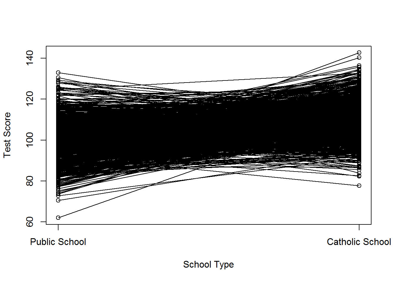
If we first assume selection into catholic school or public school (i.e. \(D_i\) is randomly assigned), we would no correlation between treatment and errors, and our simple regression correctly estimates the Average Treatment Effect. See below.
mu0 <- 100
mu1 <- 110
v0 <- rnorm(1000, mean=0, sd=10)
v1 <- rnorm(1000, mean=0, sd=10)
d <- rbinom(1000,1,.5)
y <- mu0 + (mu1 - mu0)*d + v0+d*(v1-v0)
mean(y[d==1])
## [1] 109.5076mean(y[d==0])## [1] 99.8689summary(lm(y~d))##
## Call:
## lm(formula = y ~ d)
##
## Residuals:
## Min 1Q Median 3Q Max
## -30.065 -7.007 -0.030 6.756 27.447
##
## Coefficients:
## Estimate Std. Error t value Pr(>|t|)
## (Intercept) 99.8689 0.4597 217.24 <2e-16 ***
## d 9.6387 0.6394 15.07 <2e-16 ***
## ---
## Signif. codes: 0 '***' 0.001 '**' 0.01 '*' 0.05 '.' 0.1 ' ' 1
##
## Residual standard error: 10.1 on 998 degrees of freedom
## Multiple R-squared: 0.1855, Adjusted R-squared: 0.1847
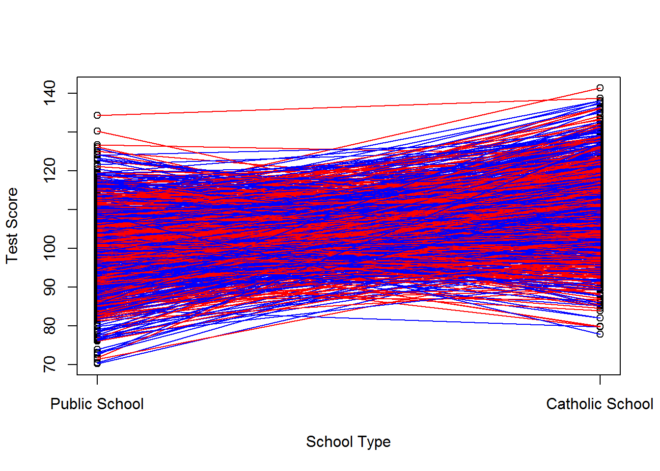
## F-statistic: 227.3 on 1 and 998 DF, p-value: < 2.2e-16cor(d, v1)## [1] 0.01110165cor(d, v0)## [1] 0.00657949cor(d, (v1-v0))## [1] 0.002837813A graphical representation is below. Red lines represent kids in catholic school, blue lines represent kids in public school. Note: our observational data would only include those scores for red dots in catholic school and blue dots in public school.
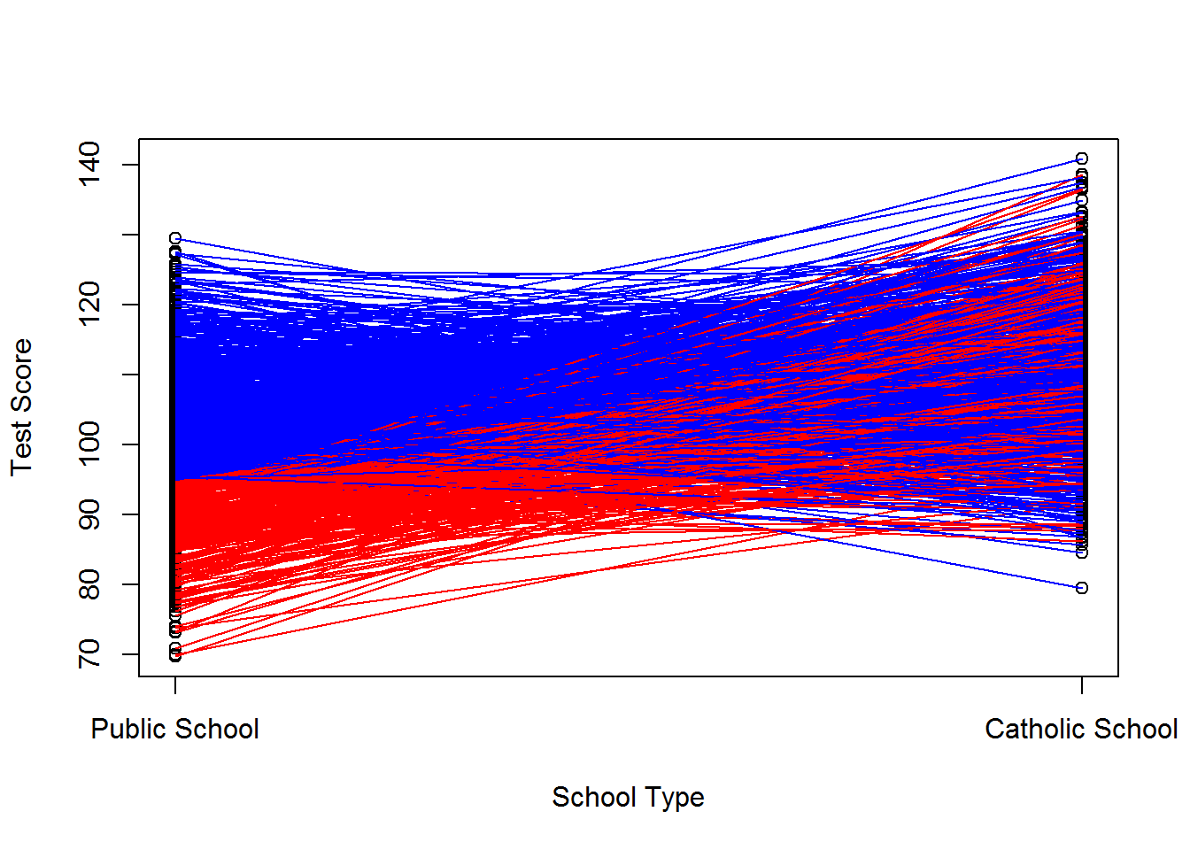
Say, instead, that public school kids with a history of bad test scores are selected to attend catholic school. Their expected \(v^0\) is less than negative 5. Further assume that these kids only underperform in publich school such that we would not expect their average deviations from \(E[v_i^1]\) to be biased, or \(E[v_i^1|D=1]=0\). We’ve now selected out the low performers from the public school population, increasing the baseline public school test scores, and left the catholic school test scores unchanged. Further, we’ve induced a correlation between \(D_i\) and \(v_i^0\) and between \(D_i\) and \(v_i^1 - v_i^0\) but not between \(D_i\) and \(v^1_i\). The estimated causal effect would be lower than the average treatment effect for this scenario. See below for the worked example.
mu0 <- 100
mu1 <- 110
v0 <- rnorm(1000, mean=0, sd=10)
v1 <- rnorm(1000, mean=0, sd=10)
d <- v0< -5
y <- mu0 + (mu1 - mu0)*d + v0+d*(v1-v0)
mean(y[d==1])
## [1] 110.7945mean(y[d==0])## [1] 104.6391summary(lm(y~d))##
## Call:
## lm(formula = y ~ d)
##
## Residuals:
## Min 1Q Median 3Q Max
## -32.863 -5.590 -0.788 5.045 28.359
##
## Coefficients:
## Estimate Std. Error t value Pr(>|t|)
## (Intercept) 104.6391 0.3064 341.5 <2e-16 ***
## dTRUE 6.1555 0.5494 11.2 <2e-16 ***
## ---
## Signif. codes: 0 '***' 0.001 '**' 0.01 '*' 0.05 '.' 0.1 ' ' 1
##
## Residual standard error: 8.042 on 998 degrees of freedom
## Multiple R-squared: 0.1117, Adjusted R-squared: 0.1108
## F-statistic: 125.5 on 1 and 998 DF, p-value: < 2.2e-16cor(d, v1)## [1] 0.04682981cor(d, v0)## [1] -0.7644251cor(d, (v1-v0))## [1] 0.5469256If we were to graph the potential outcomes, we would see the following:
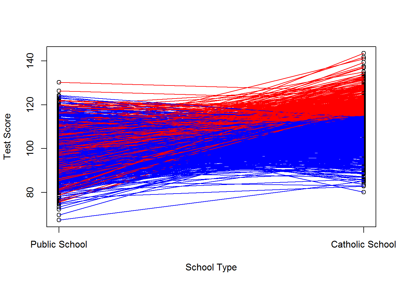
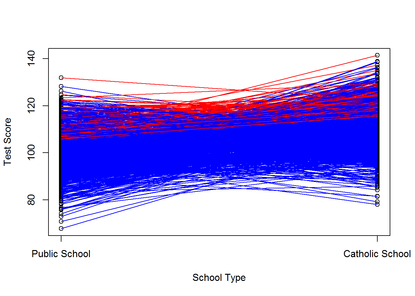
We can do the same for an example where we only select kids who we think will prosper in catholic school for treatment. We only choose those who have a \(v_i^1 > 5\), but we ignore \(v_i^0\) in our treatment assignment. We have left the baseline performance unchanged (we’ve randomly selected on \(v_i^0\) afterall), but we’ve increased the performance of catholic school children on average. We’ve thus induced a correlation between \(D_i\) and \(v_i^1\) and between \(D_i\) and \(v_i^1 - v_i^0\) but not between \(D_i\) and \(v_i^0\). See below for the worked example.
mu0 <- 100
mu1 <- 110
v0 <- rnorm(1000, mean=0, sd=10)
v1 <- rnorm(1000, mean=0, sd=10)
d <- v1 > 5
y <- mu0 + (mu1 - mu0)*d + v0+d*(v1-v0)
mean(y[d==1])
## [1] 121.1983mean(y[d==0])## [1] 100.384summary(lm(y~d))##
## Call:
## lm(formula = y ~ d)
##
## Residuals:
## Min 1Q Median 3Q Max
## -35.782 -5.257 -0.770 5.532 29.455
##
## Coefficients:
## Estimate Std. Error t value Pr(>|t|)
## (Intercept) 100.3840 0.3519 285.26 <2e-16 ***
## dTRUE 20.8144 0.6231 33.41 <2e-16 ***
## ---
## Signif. codes: 0 '***' 0.001 '**' 0.01 '*' 0.05 '.' 0.1 ' ' 1
##
## Residual standard error: 9.183 on 998 degrees of freedom
## Multiple R-squared: 0.5279, Adjusted R-squared: 0.5274
## F-statistic: 1116 on 1 and 998 DF, p-value: < 2.2e-16cor(d, v1)## [1] 0.7655565cor(d, v0)## [1] -0.02760982cor(d, (v1-v0))## [1] 0.5458536The plot of this example would look like this:
We can also select those kids who would do well in either catholic school or in public school. Say we assign treatment to those with \(v_i^0\) and \(v_i^1\) greater than 5. We’ve thus pushed down the public school scores while increasing the catholic school scores. We’ve induced a correlation between \(D_i\) and both \(v_i^0\) and \(v_i^1\) but not between \(D_i\) and \(v_i^1 -v_i^0\). See below for the worked example.
mu0 <- 100
mu1 <- 110
v0 <- rnorm(1000, mean=0, sd=10)
v1 <- rnorm(1000, mean=0, sd=10)
d <- v0 > 10 & v1 > 5
y <- mu0 + (mu1 - mu0)*d + v0+d*(v1-v0)
mean(y[d==1])
## [1] 120.3902mean(y[d==0])## [1] 99.26962summary(lm(y~d))##
## Call:
## lm(formula = y ~ d)
##
## Residuals:
## Min 1Q Median 3Q Max
## -29.878 -5.837 -0.054 5.981 32.747
##
## Coefficients:
## Estimate Std. Error t value Pr(>|t|)
## (Intercept) 99.2696 0.3029 327.70 <2e-16 ***
## dTRUE 21.1206 1.4124 14.95 <2e-16 ***
## ---
## Signif. codes: 0 '***' 0.001 '**' 0.01 '*' 0.05 '.' 0.1 ' ' 1
##
## Residual standard error: 9.356 on 998 degrees of freedom
## Multiple R-squared: 0.183, Adjusted R-squared: 0.1822
## F-statistic: 223.6 on 1 and 998 DF, p-value: < 2.2e-16cor(d, v1)## [1] 0.222786cor(d, v0)## [1] 0.3636571cor(d, (v1-v0))## [1] -0.09882348And the plot:
End Notes
Thanks to Monica Alexander who looked over an early draft.
Collected and commented code for this post can be found on my github
Morgan, Stephen L. and Christopher Winship. 2015. Counterfactuals and Causal Inference. Methods and Principles for Social Research. Second Edition. Cambridge University Press.